
How to Read a Dyno Sheet
This Dynojet sheet gives you curves, peak values, engine speed, correction, and smoothing. Reading it starts with the question the test was supposed to answer.
What did you put the car on the dyno to find out?
A dyno sheet is a graphic representation of data collected during a dynamometer test. There are many ways to digest that information, and the useful reading depends on what you are trying to deduce.
Are you using the power curve and shift recovery to work through gearing for a straight-line application? Comparing hardware before and after? Studying turbo response alongside pressure, temperature, and airflow? Holding the car at a repeatable operating point on a load-capable dyno while you study the ECU?
Those are four different tests. A peak number may matter to one of them and be almost irrelevant to another.
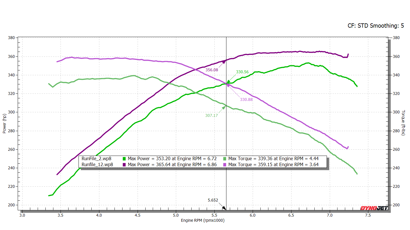
An anonymized Dynojet export. Only the third-party shop header was redacted; plotted traces, axes, correction factor, smoothing, run labels, cursor values, and peak values are unchanged.
Start with the axes, then identify the runs
Engine speed runs along the bottom in thousands of rpm. Power is read against the left axis in horsepower. Torque is read against the right axis in pound-feet. The numerical scales happen to match on this sheet, but they represent different quantities.
On this image, green represents RunFile_2.wp8 and purple represents RunFile_12.wp8. Each run has two traces: the darker line is power and the lighter line is torque. The box at the bottom gives the peak value and the engine speed where it occurred. RunFile_2 made 353.20 hp at 6,720 rpm and 339.36 lb-ft at 4,440 rpm. RunFile_12 made 365.64 hp at 6,860 rpm and 359.15 lb-ft at 3,640 rpm.
The vertical cursor is parked at 5,652 rpm. The four values printed beside it are what each trace was making at that engine speed. They are not additional peak figures.
Horsepower and torque cross numerically near 5,252 rpm when horsepower and pound-feet use the same scale because horsepower equals torque multiplied by rpm, divided by 5,252. The crossover is arithmetic. Torque can peak earlier and begin falling while horsepower keeps rising because engine speed is still increasing.
Here is the arithmetic: one horsepower equals 33,000 foot-pounds per minute. One engine revolution is 2π radians, so horsepower equals torque × 2π × rpm ÷ 33,000—usually written as torque × rpm ÷ 5,252. At 5,252 rpm, the numerical values are therefore equal.
The peak is one point in the pull
Peak horsepower is one point in the result. RunFile_12 made 12.44 more peak horsepower and 19.79 more peak torque. Its torque peak also occurred about 800 rpm earlier, and its power trace stayed above RunFile_2 through most of the pull.
Trace shape shows where torque arrives, how long the engine carries power, and where output begins to fall away. If you are thinking about acceleration, gearing, or shift recovery, the output across the rpm range you actually use can matter more than one point at the top of the sheet.
The filenames identify the runs and nothing more. Fuel, hardware, calibration, gear, ramp rate, temperatures, and the variable being tested are missing. We can measure the difference between the curves; the cause remains unknown until the run notes or supporting data are attached.
This power-only sheet is not an ECU log
This export contains horsepower and torque. Cylinder fill, requested and delivered torque, ignition correction, boost control, fuel pressure, knock response, and the rest of the ECU's control behavior require additional channels. Dynojet can record OBD and auxiliary data when the operator selects and acquires them.
For a modern torque-based ECU, the basic power curve may be one of the least interesting records produced during a serious calibration session. It documents what reached the dyno. Supporting channels can help explain how the ECU got there and whether an intervention occurred.
A load-capable Dynojet can hold or control an operating point for this kind of work. An inertia-only sweep simply accelerates through the range and cannot hold the same condition. The channels recorded determine whether you leave with only a power curve or with the supporting calibration data needed to interpret it.
Keep wheel output and crank output separate
The roller sheet shown here reports output at the tire-to-roller interface, after the drivetrain. A hub Dynojet reports output at the hubs. Neither is a direct engine-dyno measurement.
Adding a fixed drivetrain-loss percentage produces an estimate, not a measured crank figure for that vehicle. Report the roller results shown here as WHP and WTQ; identify hub-dyno results as hub horsepower and torque.
Read CF: STD and Smoothing: 5 before comparing runs
The upper-right corner says this sheet uses the STD atmospheric correction standard. The same saved pull can display a different peak when rendered as STD, SAE, or uncorrected even though the original test has not changed.
Smoothing: 5 is the highest smoothing level on this Dynojet display and shows the least short-term detail. It makes the traces easier to read and may change a displayed local peak when the original peak was a brief spike. The recorded pull remains the same.
For a direct overlay, render both run files with the same correction standard and smoothing. A shared axis scale keeps the pictures visually honest, but it has no effect on the underlying values. Comparable tests still require the same gear, ramp or load strategy, tire setup, heat state, and test procedure.
Change one thing, then control everything else
Decide what you are changing before the first pull. If hardware is the variable, do not also change the fuel or calibration. If calibration is the variable, keep the hardware, fuel, gear, run type, and test range fixed.
Procedure matters. Keep the vehicle-to-dyno setup consistent: tire pressure and tie-down on a roller dyno, or hub adapters and attachment on a hub dyno. Keep warm-up, starting temperatures, cooling airflow, and ramp or load strategy consistent as well. Repeat enough baseline and final pulls to recognize heat trend, drift, and ordinary run-to-run variation.
Render both runs with the same correction and smoothing, then keep the conditions and notes with the files. On the sheet above, we can state exactly how the output differed. Once the run notes and supporting data are missing, any explanation of the cause is a guess.